Double Pendulum

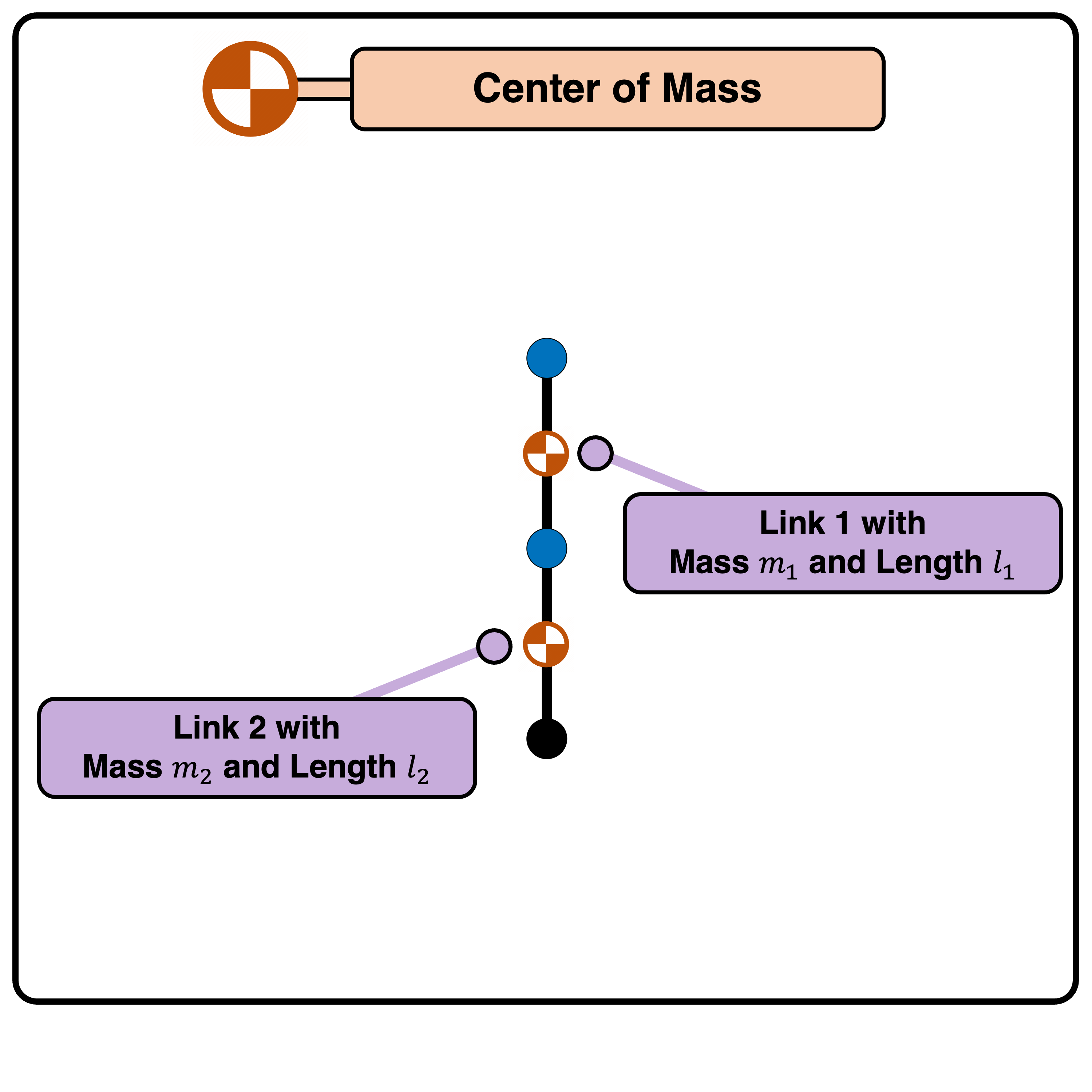
The double pendulum (often called “Acrobot”), is a heavily used example in academia. The geometric and inertial parameters are shown below:

The first link with mass \(m_1\) and length \(l_1\).
The second link with mass \(m_2\) and length \(l_2\).

Here, we assume links with uniform mass distribution.

Initial Configuration and Joint Parameters

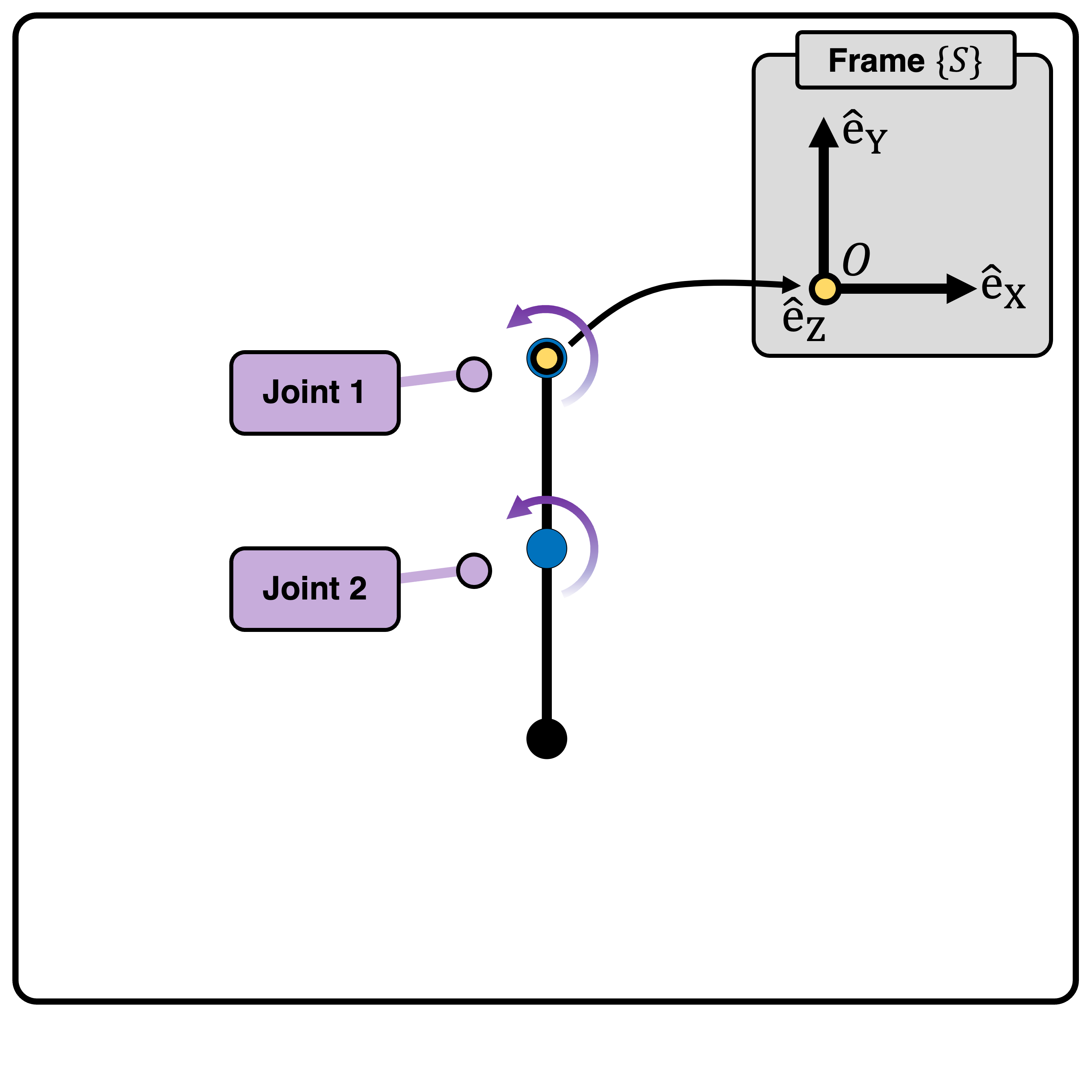
Below, the robot in initial configuration with stationary coordinate frame \(\{S\}\) and origin \(\{O\}\) is shown:

Joint	Type	Point on Joint Twist Axis (m)	Joint Direction	Joint Twist
Joint 1	Revolute (1)	(0, 0, 0)	(0, 0, 1)	(1, 0, 0, 0, 0, 0)
Joint 2	Revolute (1)	(0, \(-l_1\), 0)	(0, 0, 1)	(\(-l_1\), 0, 0, 0, 0, 1)

Example code

To construct the cart-pole robot, run the following code:

% Geometric and Inertial Parameters of the double pendulum robot
m1 = 1;         % The   mass of the  first link
m2 = 1;         % The   mass of the second link
l1 = 1;         % The length of the  first link
l2 = 1;         % The length of the second link

% Construct the double-pendulum robot and initialize
robot = DoublePendulum( m1, m2, l1, l2 );
robot.init( )

% Attach the double-pendulum robot to animation for visualization
anim = Animation( 'Dimension', 2, 'xLim', [-1.5,1.5], 'yLim', [-2.5,0.5] );
anim.init( )
anim.attachRobot( robot )

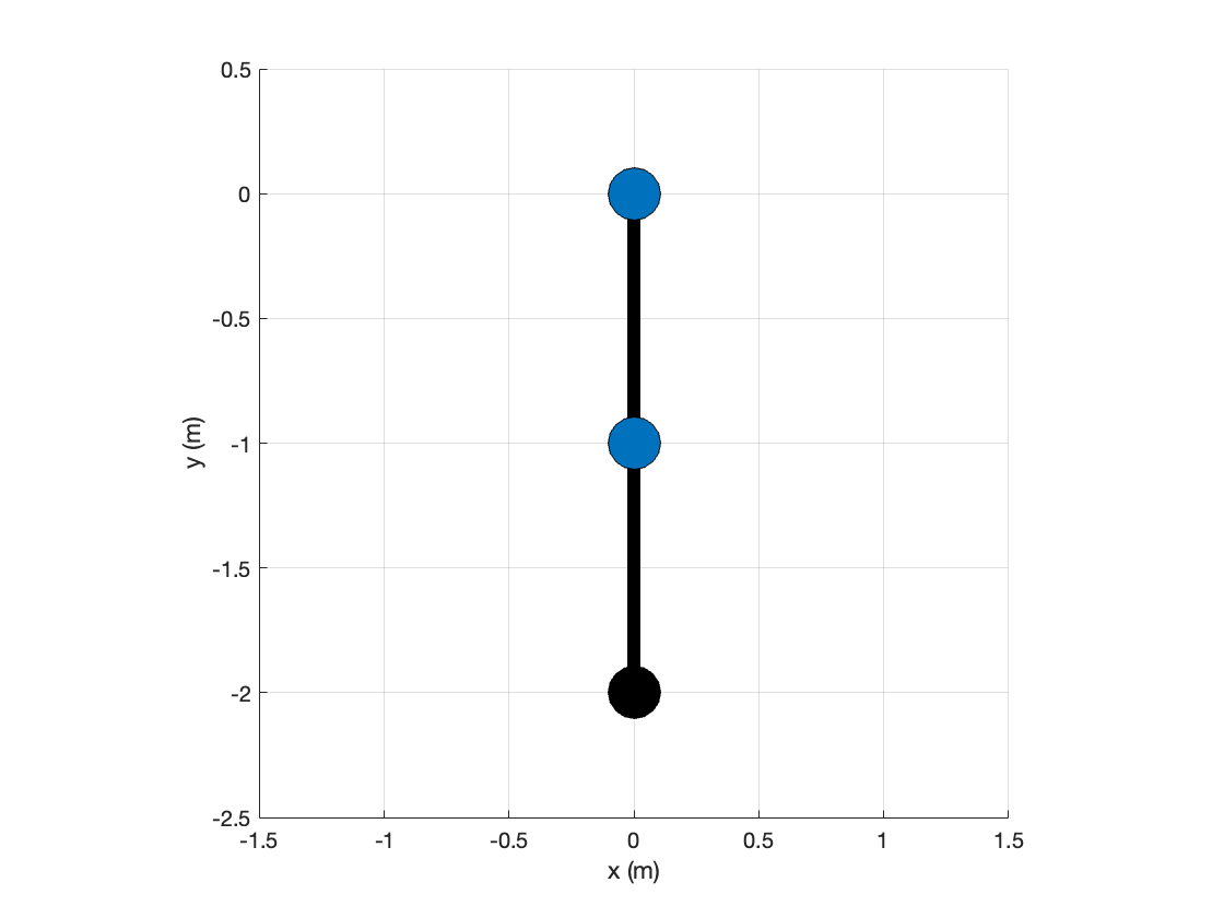
The output figure should look like this: