Franka Emika

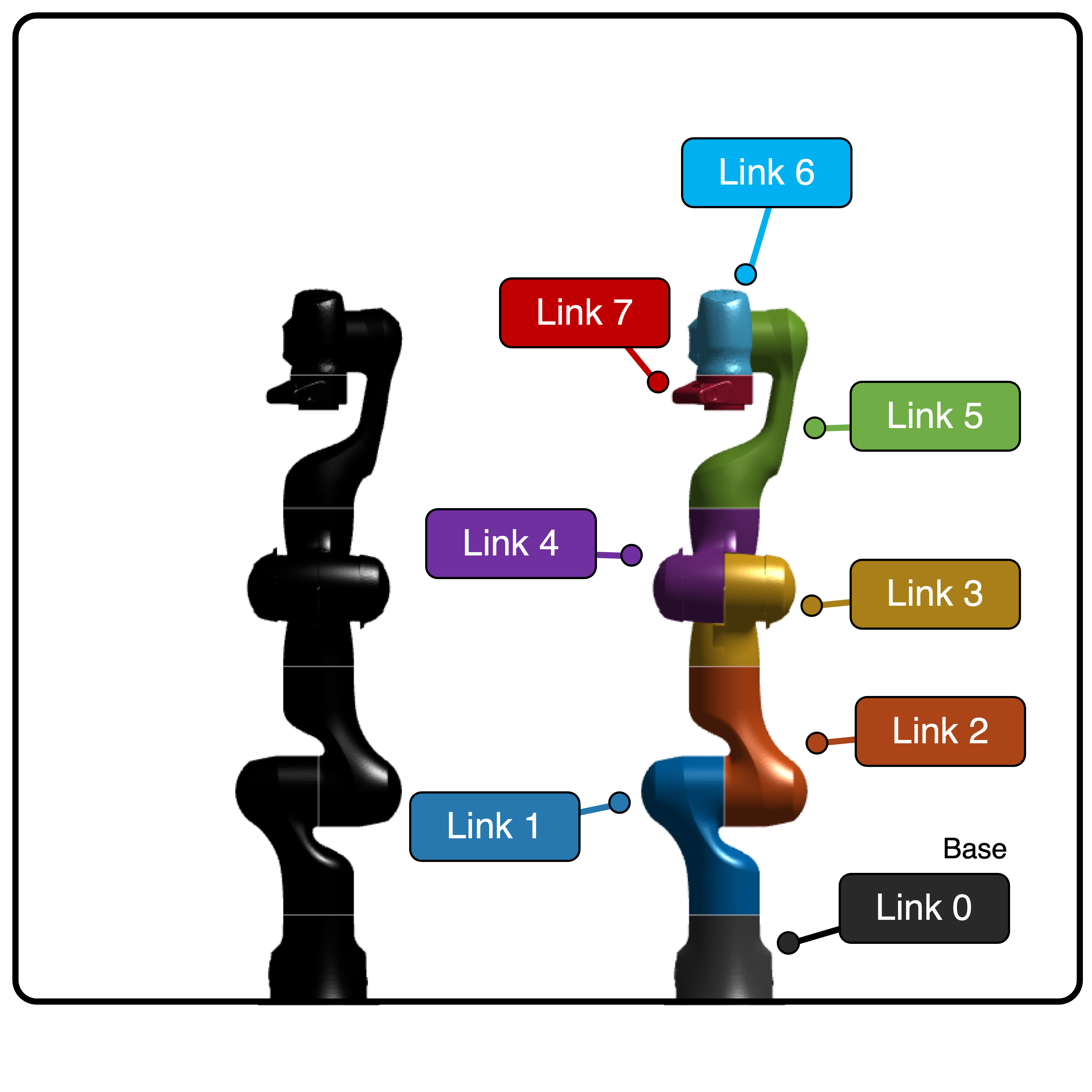
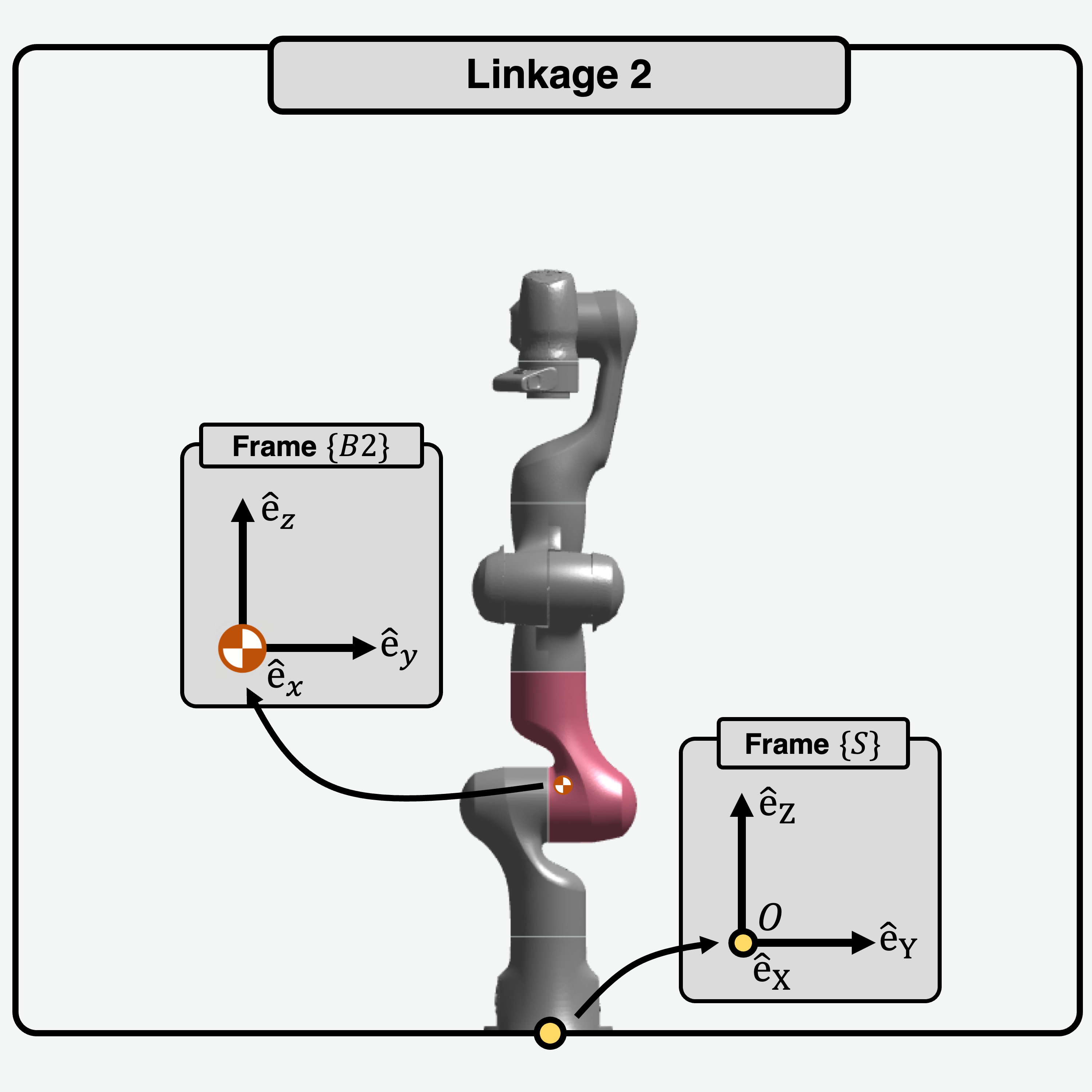
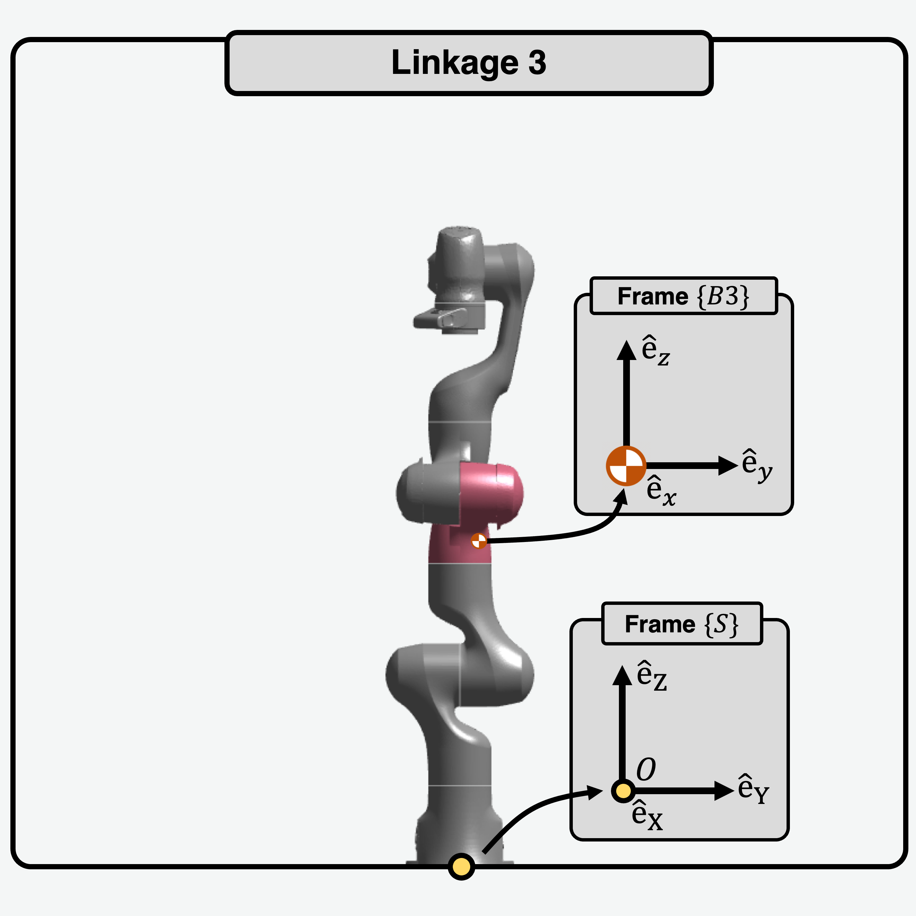
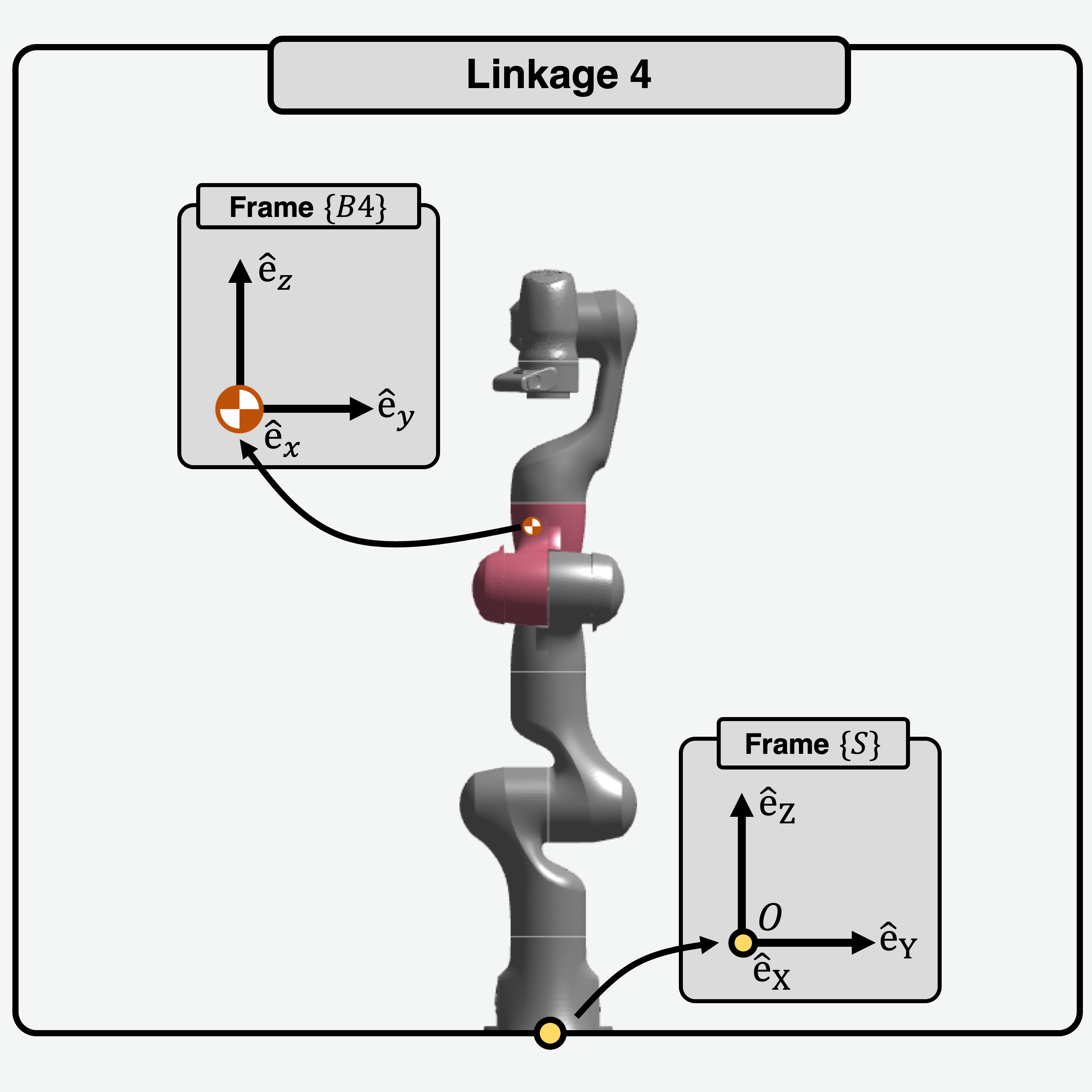
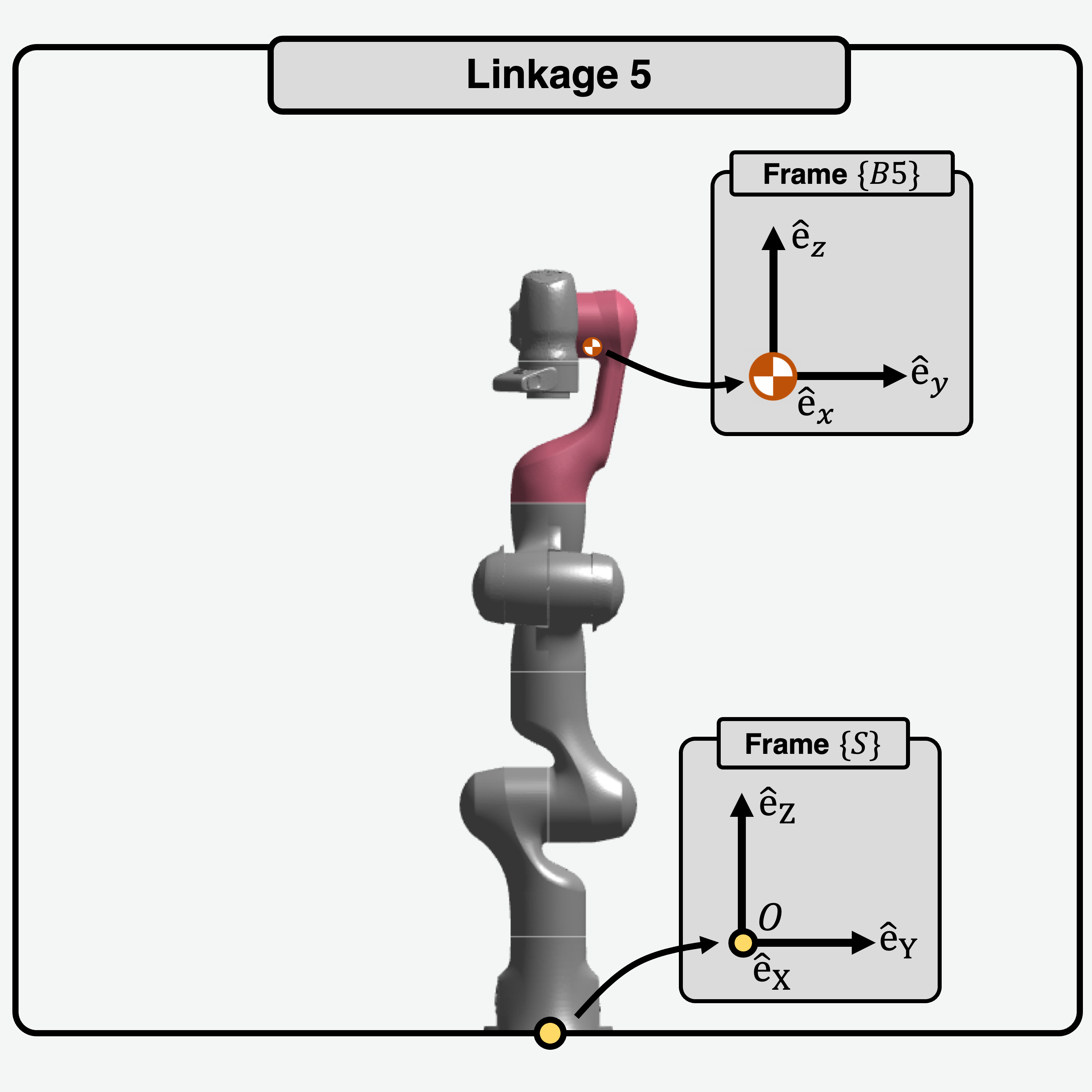
The Franka Emika Robot is a kinematically redundant robot with 7 DOF. The links and the fixed base of the robot are shown below.

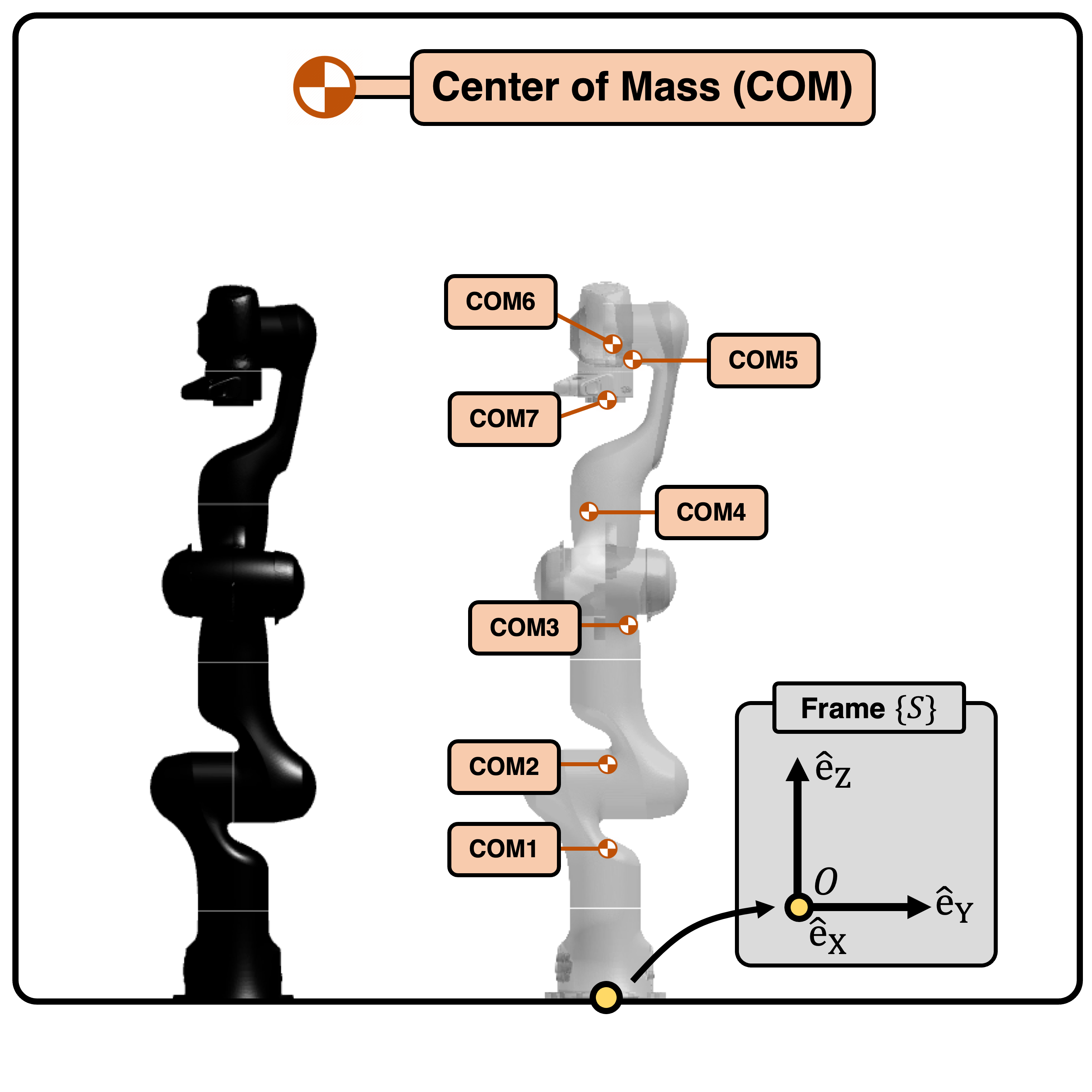
The Locations of Center of Mass (CoM)

The CoM locations of the 7 links are depicted below.

Center of Mass	Center of Mass Locations (m)	Mass (kg)
COM1	(0.0039, 0.0021, 0.2394)	4.9707
COM2	(-0.0031, 0.0036, 0.3618)	0.6469
COM3	(0.0275, 0.0392, 0.5825)	3.2286
COM4	(0.0293, -0.0275, 0.7534)	3.5879
COM5	(-0.0120, 0.0410, 0.9946)	1.2259
COM6	(0.0601, 0.0105, 1.0189)	1.6666
COM7	(0.0883, 0.0021, 0.9339)	1.4655

Note that the CoM locations are all expressed with respect to frame \(\{S\}\). The values are derived from Figure 4 in this reference. The detailed derivation of these values are shown in this post.

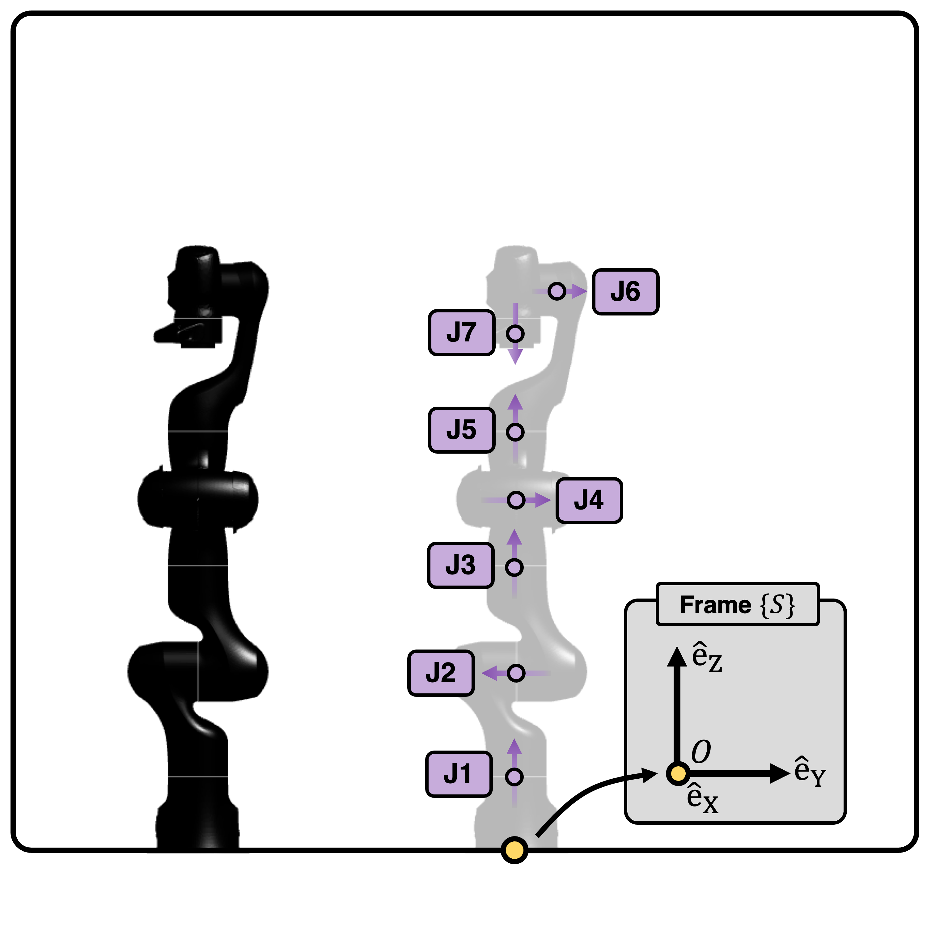
Initial Configuration and Joint Parameters

Below, the robot in initial configuration with stationary coordinate frame \(\{S\}\) and origin \(\{O\}\) is shown:

Joint	Type	Point on Joint Twist Axis (m)	Joint Direction	Joint Twist
J1	Rev. (1)	(0, 0, 0.3330)	(0, 0, 1)	(0, 0, 0, 0, 0, 1)
J2	Rev. (1)	(0, 0, 0.3330)	(0, -1, 0)	(0.333, 0, 0, 0, -1, 0)
J3	Rev. (1)	(0, 0, 0.6490)	(0, 0, 1)	(0, 0, 0, 0, 0, 1)
J4	Rev. (1)	(0.0825, 0, 0.6490)	(0, 1, 0)	(-0.649, 0, 0.0825, 0, 1, 0)
J5	Rev. (1)	(0, 0, 1.0330)	(0, 0, 1)	(0, 0, 0, 0, 0, 1)
J6	Rev. (1)	(0, 0, 1.0330)	(0, 1, 0)	(-1.0330, 0, 0, 0, 1, 0)
J7	Rev. (1)	(0.0880, 0, 1.0330)	(0, 0, -1)	(0, 0.0880, 0, 0, 0, -1)

Here, “Rev.”” stands for revolute joint.

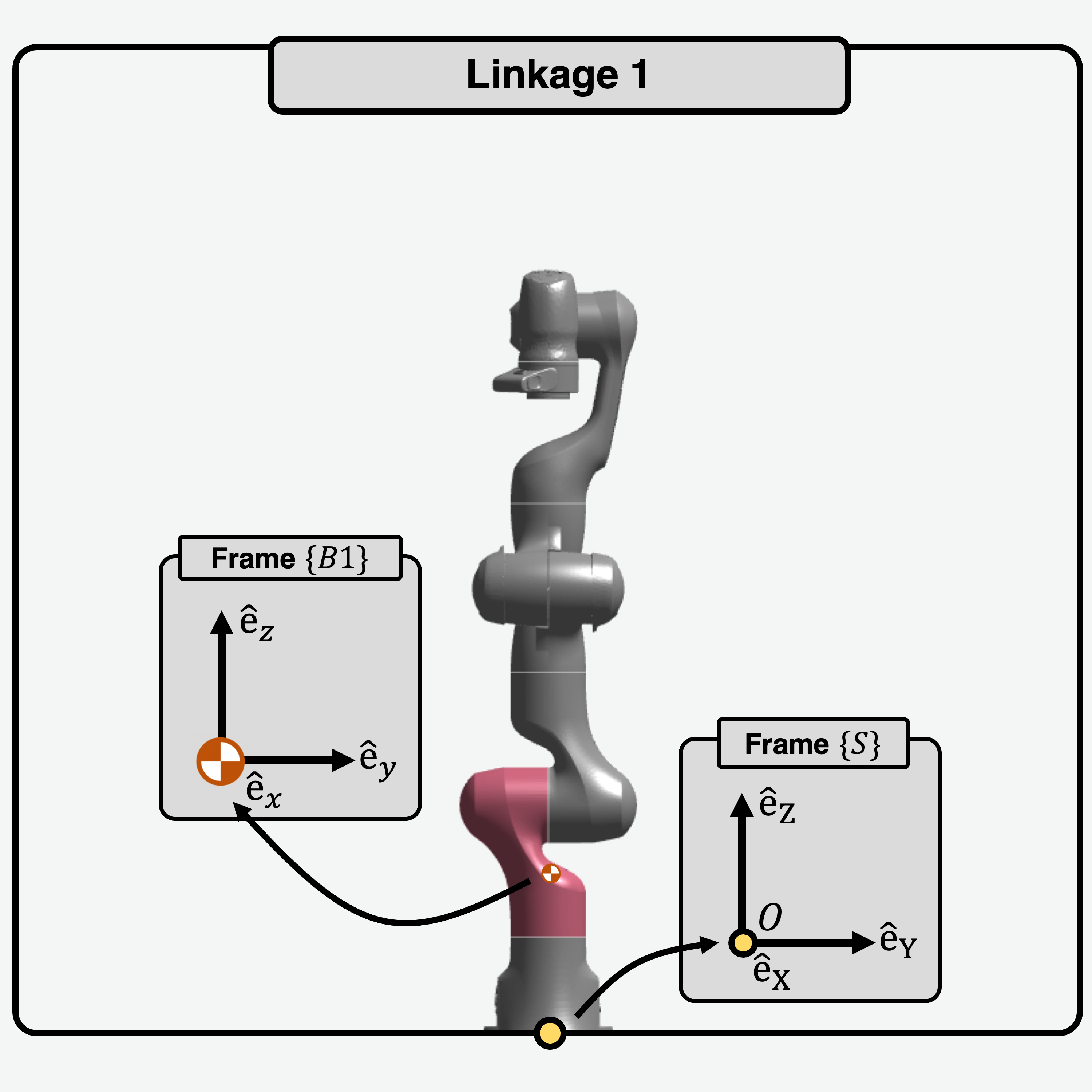
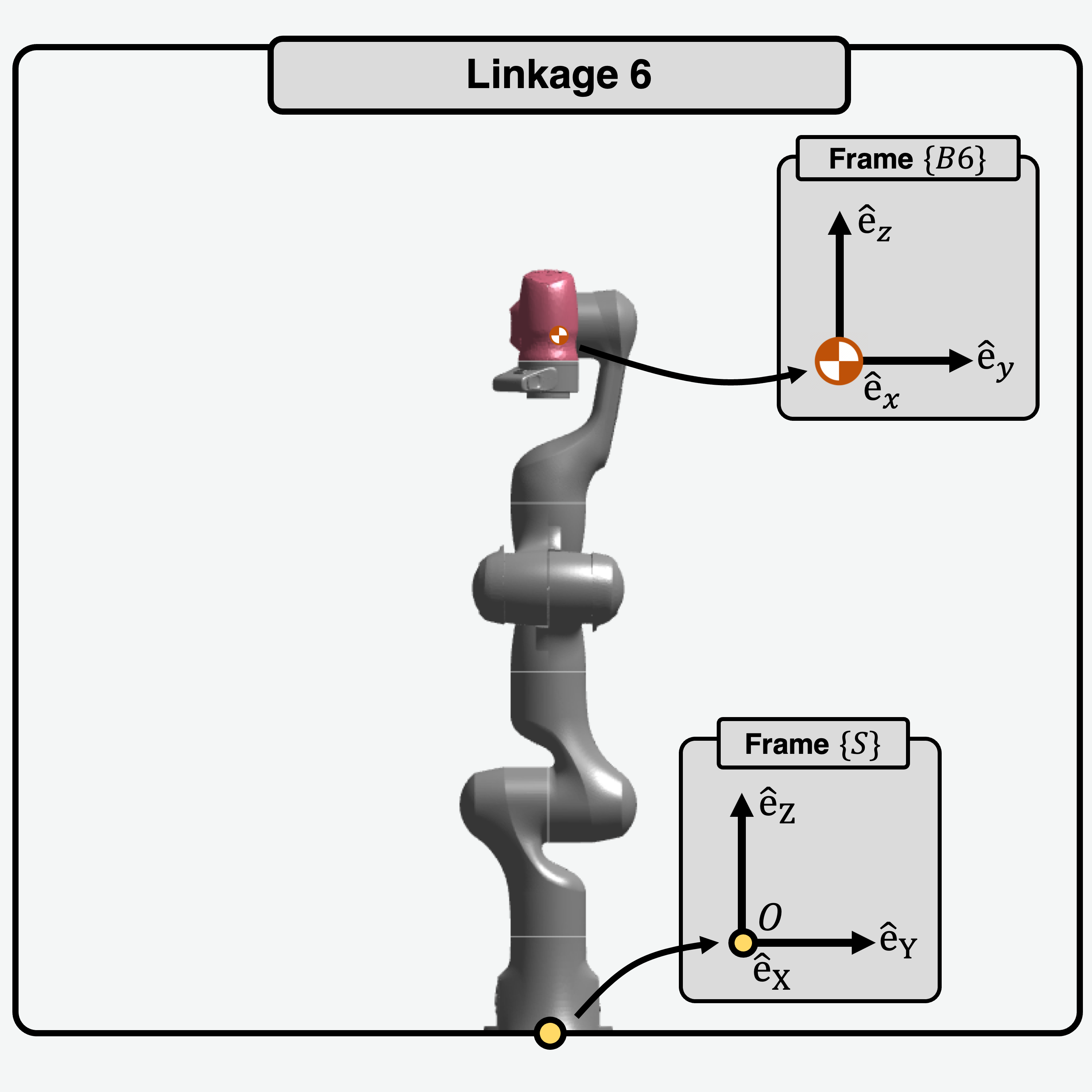
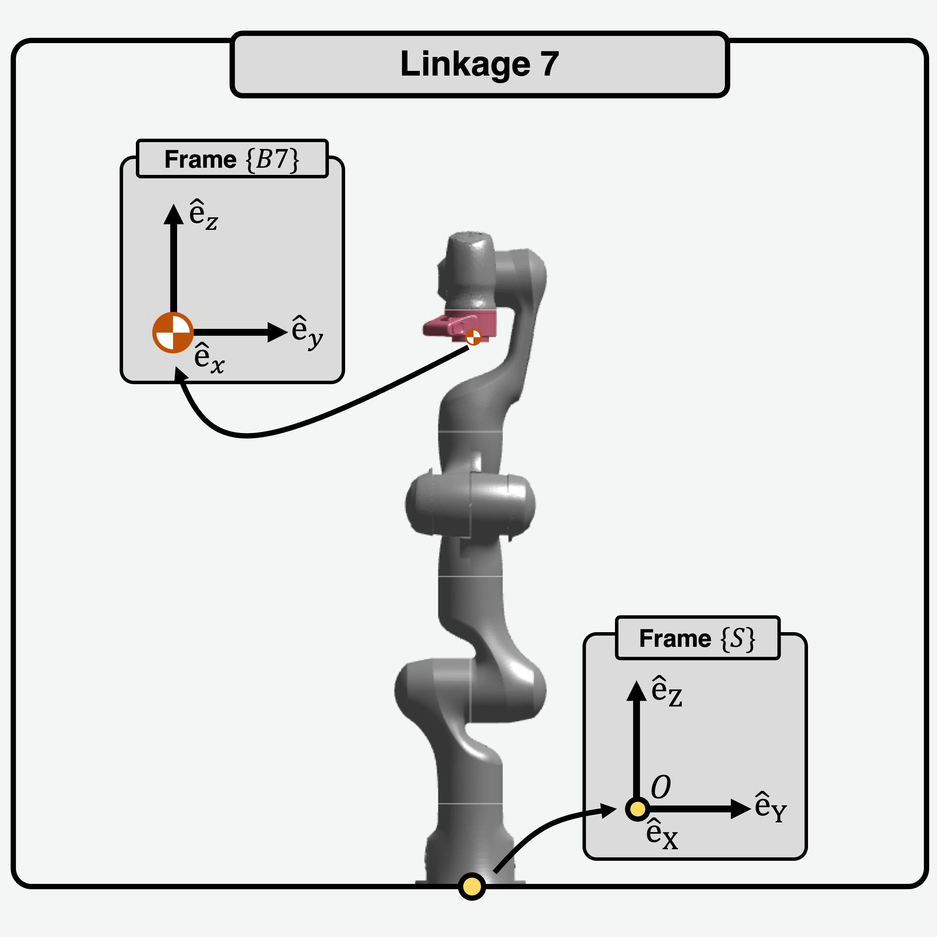
Inertia Tensor of each Linkage

Given axes \(\hat{e}_x\), \(\hat{e}_y\), \(\hat{e}_z\), the inertia matrices of the links about the CoM, \(I_i\) are shown below:

\[\begin{split}I_{1} = \begin{bmatrix} \phantom{-}0.7470 & -0.0002 & 0.0086 \\ -0.0002 & \phantom{-}0.7503 & 0.0201 \\ \phantom{-}0.0086 & \phantom{-}0.0201 & 0.0092 \end{bmatrix}\end{split}\]

\[\begin{split}I_{2} = \begin{bmatrix} 0.0085 & \phantom{-}0.0103 & \phantom{-}0.0040 \\ 0.0103 & \phantom{-}0.0265 & -0.0008 \\ 0.0040 & -0.0008 & \phantom{-}0.0281 \end{bmatrix}\end{split}\]

\[\begin{split}I_{3} = \begin{bmatrix} \phantom{-}0.0565 & -0.0082 & -0.0055 \\ -0.0082 & \phantom{-}0.0529 & -0.0044 \\ -0.0055 & -0.0044 & \phantom{-}0.0182 \end{bmatrix}\end{split}\]

\[\begin{split}I_{4} = \begin{bmatrix} \phantom{-}0.0677 & -0.0039 & 0.0277 \\ -0.0039 & \phantom{-}0.0776 & 0.0016 \\ \phantom{-}0.0277 & \phantom{-}0.0016 & 0.0324 \end{bmatrix}\end{split}\]

\[\begin{split}I_{5} = \begin{bmatrix} \phantom{-}0.0394 & -0.0015 & -0.0046 \\ -0.0015 & \phantom{-}0.0315 & \phantom{-}0.0022 \\ -0.0046 & \phantom{-}0.0022 & \phantom{-}0.0109 \end{bmatrix}\end{split}\]

\[\begin{split}I_{6} = \begin{bmatrix} 0.0025 & \phantom{-}0.0001 & \phantom{-}0.0015 \\ 0.0001 & \phantom{-}0.0118 & -0.0001 \\ 0.0015 & -0.0001 & \phantom{-}0.0106 \end{bmatrix}\end{split}\]

\[\begin{split}I_{7} = \begin{bmatrix} \phantom{-}0.0308 & -0.0004 & \phantom{-}0.0007 \\ -0.0004 & \phantom{-}0.0284 & -0.0005 \\ \phantom{-}0.0007 & -0.0005 & \phantom{-}0.0067 \end{bmatrix}\end{split}\]

The values are derived from Figure 4 of this reference. The detailed derivation of these values are shown in this post.

Example Exp[licit]-MATLAB

To construct a Franka robot in Exp[licit]-MATLAB, run the following code:

% Construct Franka object, with high visual quality
robot = franka(  );
robot.init( );

% Set figure size and attach robot for visualization
anim = Animation( 'Dimension', 3, 'xLim', [-0.7,0.7], 'yLim', [-0.7,0.7], 'zLim', [0,1.4] );
anim.init( );
anim.attachRobot( robot )

The output figure should look like this:

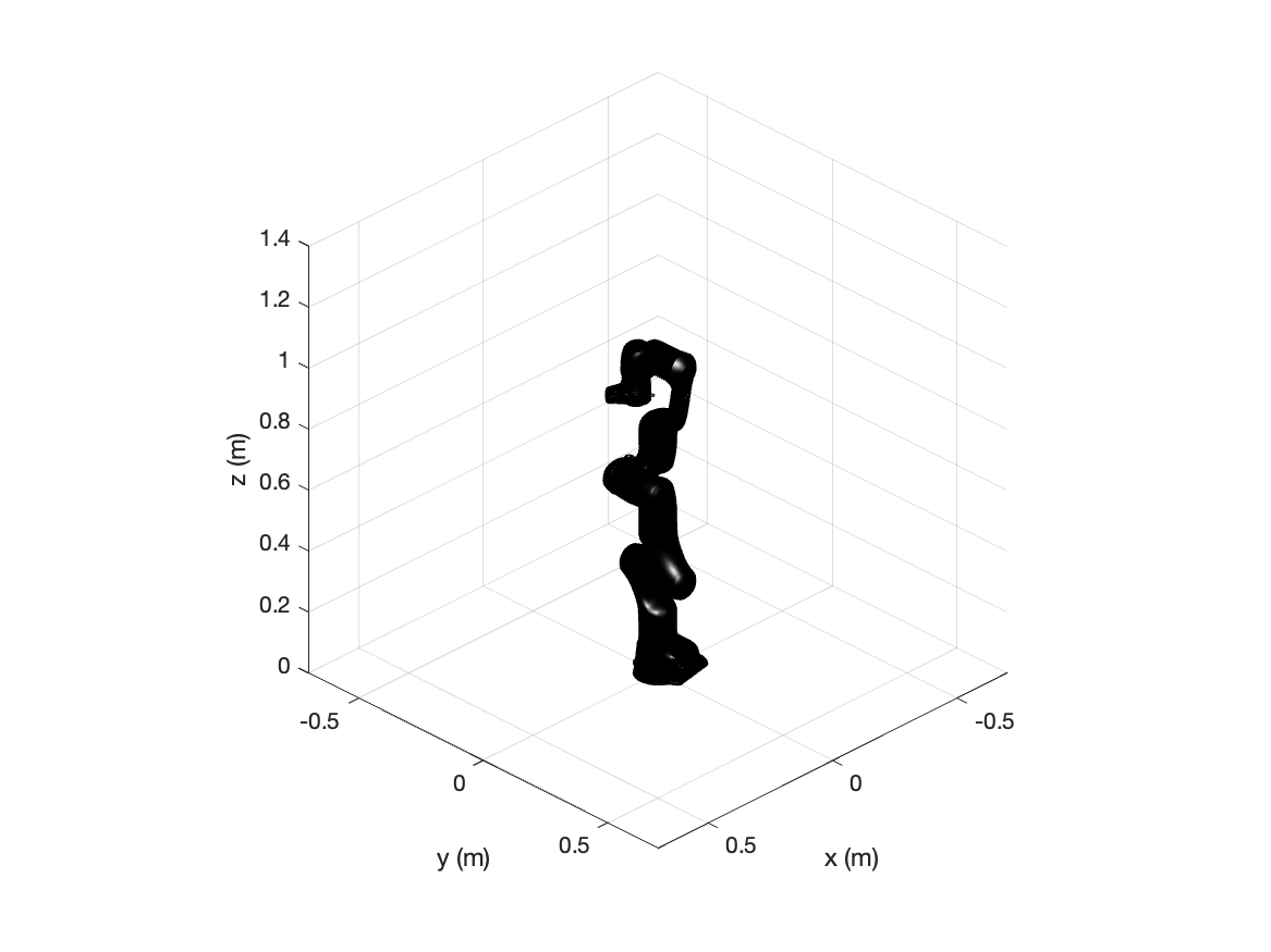
An example application for the Franka robot can be found under /examples/main_franka.m.